Merger Arbitrage in the US

options(tz="America/New_York")
Sys.setenv(TZ="America/New_York")
Economic Rational
Hedge Funds are active investors using market opportunities in their advantage. To earn high returns, they focus on one or more market strategies. One of the event driven strategies that hedge funds rely on is Risk Arbitrage (or differently Merger Arbitrage). The rationale of this strategy is to take advantage of expected price movements of target company’s share after the announcement of merger or acquisition.
The target company’s shares trade for less than the merger consideration’s per-share value—a spread that compensates the investor for the risk of the transaction not closing, as well as for the time value of money until closing. This spread does not come riskless, because there is always a chance that the merger won’t take place, leading to decline in target’s price and subsequently losses for hedge funds. The idea of the risk arbitrage strategy is to immediately after announcement of merger or acquisition, the investor should buy the stock of the target company and short sell the stock of the acquiring company.
The best way to show potential benefits of this strategy is via an example. We can think of company A with stock price of 25 GBP. Afterwards there is a press conference where company B announces it wants to acquire company A at the price of 50 GBP. After the press release, as markets are efficient, the stock price of A rises but not to full acquisition stock price of 50, but a little less than that. The stock price does not rise to 50 but only to 40 for example, because of the risk that the acquisition won’t take place. So, markets are saying there is a 80% chance the merger will succeed.
The merger may not go ahead as planned because of conditional requirements from one or both companies, or regulations may eventually prohibit the merger for monopoly or funding reasons. Those who take part in this kind of strategy must, therefore, be fully knowledgeable about all the risks involved as well as the potential rewards. Because merger arbitrage comes with uncertainty, hedge fund managers must fully evaluate these deals and accept the risks that come with this kind of strategy.
The deal can go as a stock deal or cash deal. If we consider a cash deal, in our example it means company B will pay 50 GBP to every share of company A. Investors that are long in company A’s stocks makes a profit (50 – 40 GBP) out of risk arbitrage.
If the deal is a stock deal, in essence we can think of a scenario that company B is willing to issue 2 million shares and give it to shareholders of company A (with 1 million shares outstanding). After thes tock deal, only stocks left on the market will be of company B receiving control on merged company. In essence, shareholders of company B are giving two shares of company B to one share of company A.
Theoretically, if we expect the merger to go through, at whatever price company B’s stock is trading, A should trade at double that price. The rationale is that an investor will be able to trade one share of company A for 2 shares of company B after the deal completes. If share of company A is not trading at double of the share price of company A, there exists risk arbitrage, as some investors think there is probability that the merger will not succeed. In a stock deal, an investor can protect her/himself of both systematic and unsystematic risk.
The idea is that if the market goes down, both stocks can follow the market movements (assuming beta >0), but even in that case investor can earn positive riskless profits. The best way to assure profits is to set up a pair trade. Investor should go long one share of company A and simultaneously short two shares of company B. The reason this works is if investor knows the transaction is going to happen two shares of company B will be worth more than two shares of company A.
So, when investor shorts two shares of B (if we think share of B is trading at price of 25 GBP) this means we get 50 GBP by short selling two stock of B.
Simultaneously an investor buys stock of company A that is trading at 40 GBP (cost of 40 GBP). Assuming the transaction happens, at some future date, one share of company A an investor has can be traded for two shares of B and an investor uses these two shares to cover its short position. The net profit of the transaction turns out to be 10 GBP if the deal goes through.
In reality, there are other ways an investor can trade on merger arbitrage, such as covering his long position with an put option on acquirers stock, but in this project we have focused on merger arbitrage of going long on the target company’s stock and going short on the acquirer’s stock with stock deal.
Data Collection
To test our economic rational, we decided to look at the spread of stock returns of both acquirer and target companies between the announcement day of a new M&A deal and its closure or withdrawal. We then investigated what returns this would create for a strategy that longs the target stock and shorts the acquirer, both on a day to day basis and cumulative. Finally, we tested our trading strategy in a time series and compared it to the market. As mentioned in the previous section we identified 348 M&A deals in the USA between 2010 and 2020 of which we successfully collected stock price data of both target and acquirer for 104 deals (>30%).
Benchmark data
Risk-free Rates
tbill <- vroom("https://fred.stlouisfed.org/graph/fredgraph.csv?bgcolor=%23e1e9f0&chart_type=line&drp=0&fo=open%20sans&graph_bgcolor=%23ffffff&height=450&mode=fred&recession_bars=on&txtcolor=%23444444&ts=12&tts=12&width=1168&nt=0&thu=0&trc=0&show_legend=yes&show_axis_titles=yes&show_tooltip=yes&id=DTB3&scale=left&cosd=2009-08-01&coed=2020-10-09&line_color=%234572a7&link_values=false&line_style=solid&mark_type=none&mw=3&lw=2&ost=-99999&oet=99999&mma=0&fml=a&fq=Daily&fam=avg&fgst=lin&fgsnd=2020-02-01&line_index=1&transformation=lin&vintage_date=2020-10-14&revision_date=2020-10-14&nd=1954-01-04") %>%
  mutate(DTB3 = DTB3/100) %>%
  rename("date" = "DATE",
         "T_bill" = "DTB3") %>%
  mutate(T_bill_d = (1 + T_bill)^(1/252)-1,
         date = as.Date(date,"%Y-%m-%d"))
Indices
benchmark <-
  data.frame(index = c("MNA", "^RUA", "^FTSE","^FTAS", "^IXIC","NYA", "^DJI", "^GSPC"),
             description = c("IQ Merger Arbitrage ETF", "Russell_3000", "FTSE 100", "FTSE All Share","NASDAQ_Composite", "NYSE Composite", "Dow Jones Industrial Average", "SP_500")) %>%
  tq_get(get  = "stock.prices",
         from = "2009-01-01",
         to   = "2020-08-31") %>%
  select(index, description, date, close) %>%
  group_by(index) %>%
  mutate(index_return = close/lag(close) - 1)
Merger Data
Merger Deals
stocks2 <- read_excel("MA_vF.xlsx", sheet = "Sheet1") %>%
  select(acquirer, target, DealStatus, announce_date, close_date) %>%
  mutate(DealStatus = case_when(
    DealStatus == "Completed" ~ DealStatus,
    TRUE ~ "Failed"),
    DealID = paste(acquirer,target))
Get Stock Data and build Dataframes
To create our data set we used the acquired deal data from Bloomberg and downloaded the respective companies’ opening stock prices from Yahoo Finance. Here a big part of the data got lost due to the nature of Yahoo Finance stopping to track stocks that are no longer traded. As companies that have been acquired do no longer trade their shares, we have poor data quality for the target data set.
Acquirer Data
acquirer_raw <- stocks2 %>%
  select(acquirer) %>%
  tq_get(get  = "stock.prices",
         from = "2009-01-01",
         to   = "2020-08-31") %>%
  select(date, acquirer, open, close)
Target Data
target_raw <- stocks2 %>%
  select(target) %>%
  tq_get(get  = "stock.prices",
         from = "2009-01-01",
         to   = "2020-08-31") %>%
  select(date, target, open, close)
Reformat
# Reformat acquirer data
stock_data_acquirer <- acquirer_raw %>%
  group_by(acquirer) %>%
  mutate(close_acquirer = sprintf("%.2f", open, na.rm = TRUE)) %>%
  select(acquirer, date, close_acquirer)
# Reformat target data
stock_data_target <- target_raw %>%
group_by(target) %>%
mutate(close_target = sprintf("%.2f", open, na.rm = TRUE)) %>%
select(target, date, close_target)Trade from 1 day past announcement date
The next step was to create a coherent data frame that lists the relevant dates and stock prices for our individual deals. We then added a new column called “period” to track the days from announcement. Due to the nature of stocks only being traded on business days but deal announcement also being made over the weekends or on bank holidays we did not always have a stock price on the announcement day. We decided to shift all announcement days to the next business day.
acq_tar <- stocks2 %>%

  #Add acquirer data
  left_join(stock_data_acquirer, by = c("acquirer")) %>%
  distinct(DealID, date, .keep_all = T) %>%
  mutate(announce_date = as.Date(announce_date,"%Y-%m-%d", tz = "America/New_York"),
         close_date = as.Date(close_date,"%Y-%m-%d", tz = "America/New_York"),
         standard_date = date - announce_date,
         standard_date2 = lead(standard_date, n = 2L)) %>%
  group_by(DealID) %>%
  filter(standard_date >= -2,
         date <= close_date) %>%
  mutate(period = row_number(),
         period = period + as.numeric(time_length( min(standard_date), "days")) -2 ) %>%

  # Add target data
  left_join(stock_data_target, by = c("target", "date")) %>%
  drop_na(close_target) %>%

  # Add Acquirer Returns
  group_by(DealID) %>%
  mutate(close_acquirer = as.numeric(close_acquirer, na.rm = TRUE),
    ret_acq = ifelse(period < 0, NA, ifelse(period > 0, close_acquirer/lag(close_acquirer) - 1, 0))) %>%

  # Add target Returns
  group_by(DealID) %>%
  mutate(close_target = as.numeric(close_target, na.rm = TRUE),
    ret_tar = ifelse(period < 0, NA, ifelse(period > 0, close_target/lag(close_target) - 1, 0))) %>%

  # Add combined returns

  mutate(ret_combined =  ifelse(is.na(ret_tar),NA, ifelse(is.na(ret_acq),NA, ret_tar - ret_acq))) %>%
  # mutate(ret_combined = ifelse(DealStatus == "Completed", ret_tar - ret_acq,  ret_acq - ret_tar)) %>% # If predict deal succeeds vs predict deal fails, assuming 100% predictive capabilities - CAN CHANGE
  # Get rid of non-sense returns
  filter(!is.infinite(ret_combined))
Daily Return and Acquirer - Target Spread
To investigate the stock return spread between targets and acquirers in M&A deals we then calculated the mean daily returns for all targets and acquirers per period from announcement day. We found that in the early days after an announcement the target’s stocks tends to outperform the acquirer and achieves a positive return. The acquirer’s stock on the other hand often suffers from negative returns. As can be seen in the chart below this spread quickly vanishes and is predominantly kept alive by some sporadic high returns of targets in our data set.
acq_tar %>%
  group_by(period) %>%
  # Summarise means per period whilst removing all NAs. Bad data quality forces us to do this
  summarise(mean_acq = mean(ret_acq, na.rm = TRUE),
            mean_tar = mean(ret_tar, na.rm = TRUE),
            mean_strat = mean(ret_combined, na.rm = TRUE)) %>%
  filter(period <= 50) %>%
  ggplot() +
  theme_bw() +
  geom_line(aes(x = period, y = (mean_acq)), colour = "red") + # Acquirer return
  geom_line(aes(x = period, y = (mean_tar)), colour = "blue") + # Target return

  labs(title = "Return spread between Target and Acquirer narrows quickly",
       subtitle = "Mean Daily Returns of Targets and Acquirers per Day from Announcement",
       y = "Daily Returns",
       x = "Day from initial announcement") +
  theme_economist_white()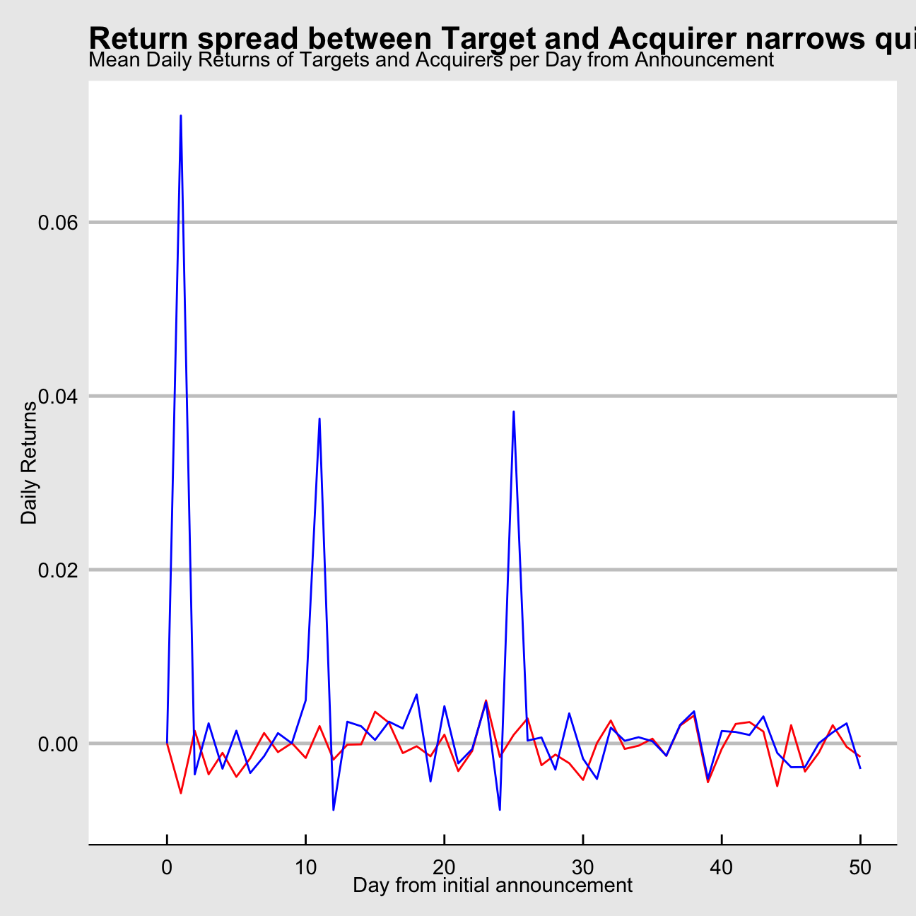
ggsave("Return Spread Target an Acquirer.png",
       plot = last_plot(),
       scale = 1,
       width = 20,
       height = 15,
       units = "cm",
       dpi = 300,
       limitsize = TRUE)

knitr::include_graphics(here::here("Return Spread Target an Acquirer.png"), error = FALSE)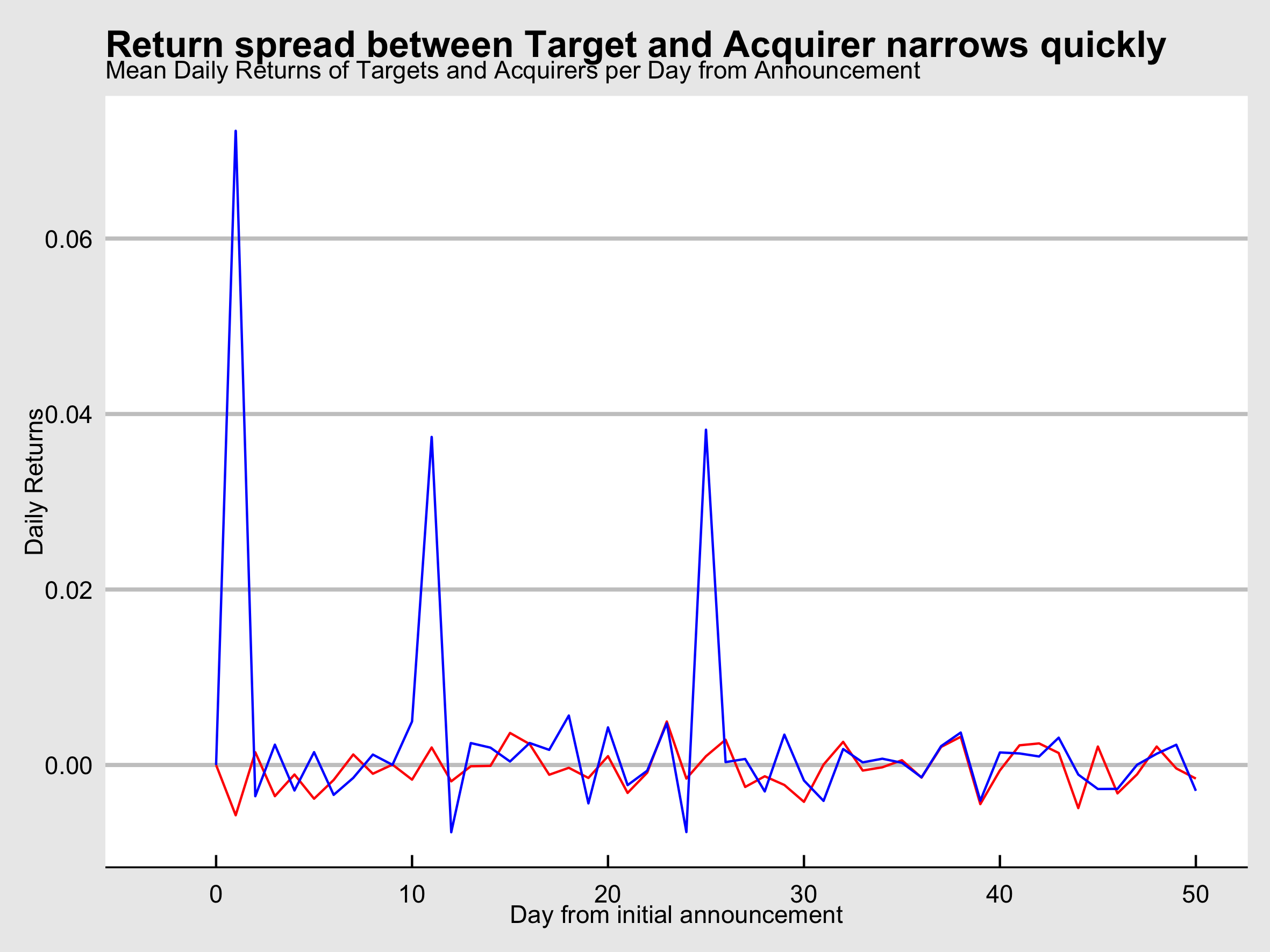
acq_tar %>%
  group_by(period) %>%
  # Summarise means per period whilst removing all NAs. Bad data quality forces us to do this
  summarise(mean_acq = mean(ret_acq, na.rm = TRUE),
            mean_tar = mean(ret_tar, na.rm = TRUE),
            mean_strat = mean(ret_combined, na.rm = TRUE)) %>%
  filter(period <= 50) %>%
  ggplot() +
  theme_bw() +
  geom_line(aes(x = period, y = (mean_strat)), colour = "green") + # Portfolio
  labs(title = "Target and Acquirer Spread drives Strategy Return",
       subtitle = "Mean Daily Returns of Strategy per Day from Announcement",
       y = "Daily Returns",
       x = "Day from initial announcement") +
  theme_economist_white()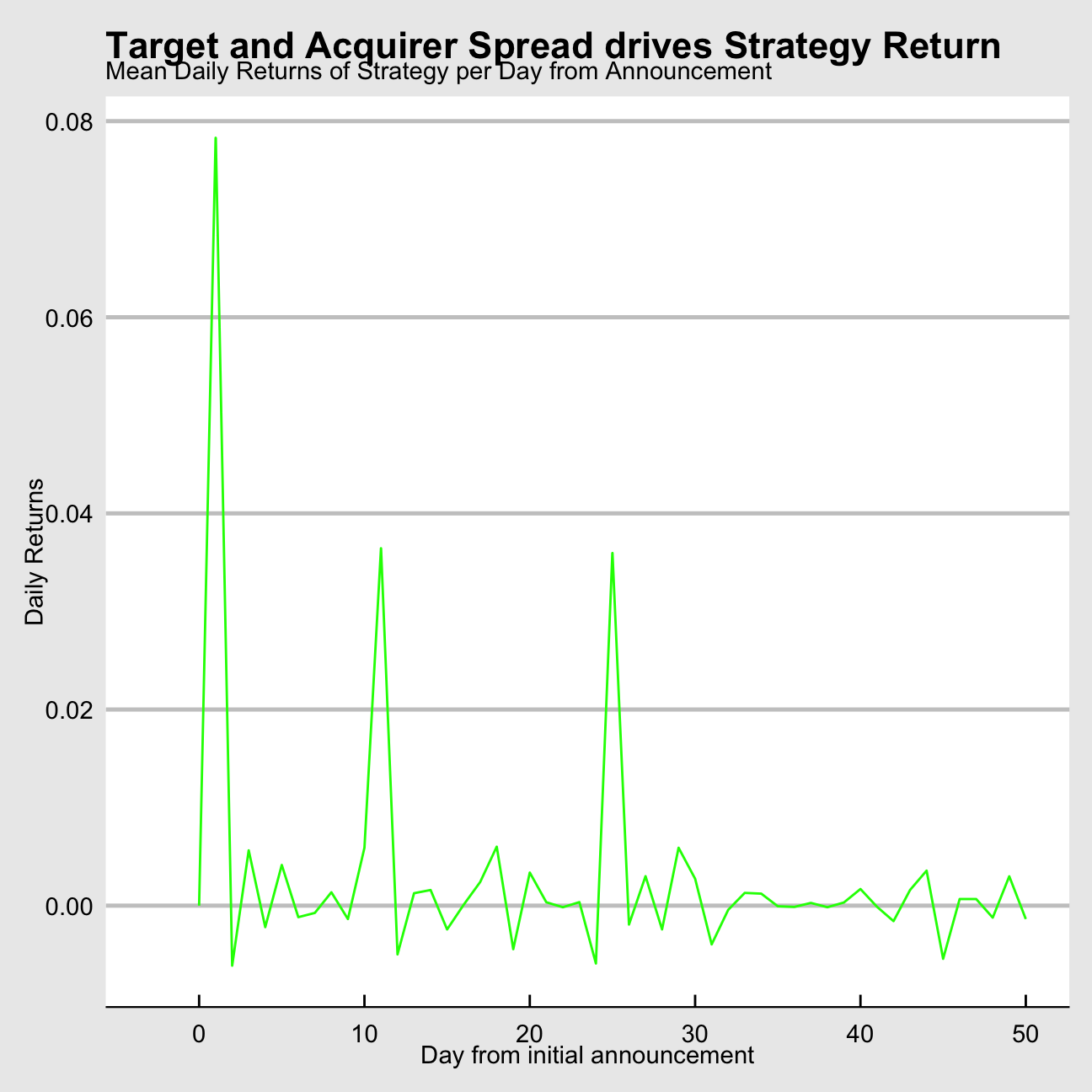
ggsave("Strategy Return from Spread.png",
       plot = last_plot(),
       scale = 1,
       width = 20,
       height = 15,
       units = "cm",
       dpi = 300,
       limitsize = TRUE)

knitr::include_graphics(here::here("Strategy Return from Spread.png"), error = FALSE)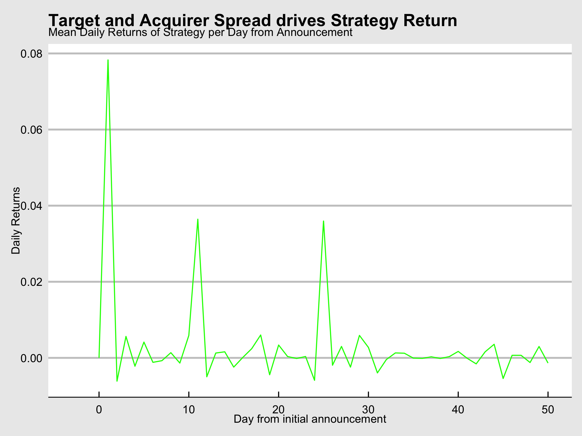
Cumulative Return
To put the previously discovered spread in daily returns into more context we calculated the average cumulative returns of both acquirers and targets over time. We then calculated the mean cumulative return of all targets and acquirers per period p.
Acquirer
# Cumulative return for acquirer
initial_acq <- acq_tar %>%
  filter(period == 0) %>%
  rename(initial_acq = close_acquirer) %>%
  select(acquirer, target, initial_acq) %>%
  distinct()

cum_acq <- left_join(acq_tar, initial_acq, by = c("acquirer", "target")) %>%
  mutate(cum_ret_acq = ifelse(period > -1, close_acquirer/initial_acq - 1, NA)) %>%
  group_by(period) %>%
  summarise(mean_cum_ret_acq = mean(cum_ret_acq, na.rm =TRUE)) %>%
  filter(period <= 50)
Target
# Cumulative return for target
initial_tar <- acq_tar %>%
  filter(period == 0) %>%
  rename(initial_tar = close_target) %>%
  select(acquirer, target, initial_tar) %>%
  distinct()

cum_tar <- left_join(acq_tar, initial_tar, by = c("acquirer", "target")) %>%
  mutate(cum_ret_tar = ifelse(period > -1, close_target/initial_tar - 1, NA)) %>%
  group_by(period) %>%
  summarise(mean_cum_ret_tar = mean(cum_ret_tar, na.rm =TRUE)) %>%
  filter(period <= 50)
Cumulative Return Spread
# Combine all
cum_all <- left_join(cum_acq, cum_tar, by = "period") %>%
  filter(period <= 50)


ggplot(cum_all) +

  geom_line(aes(x = period, y = mean_cum_ret_tar), colour = "blue") +
  geom_line(aes(x = period, y = mean_cum_ret_acq), colour = "red") +
  theme_bw() +
  labs(subtitle = "Mean Cumulative Return - Investments start 1 day after announcement",
       title = "Target outperformance in cumulative return driven by early gains",
       y = "Cumulative Return",
       x = "Day from announcement") +
  theme_economist_white()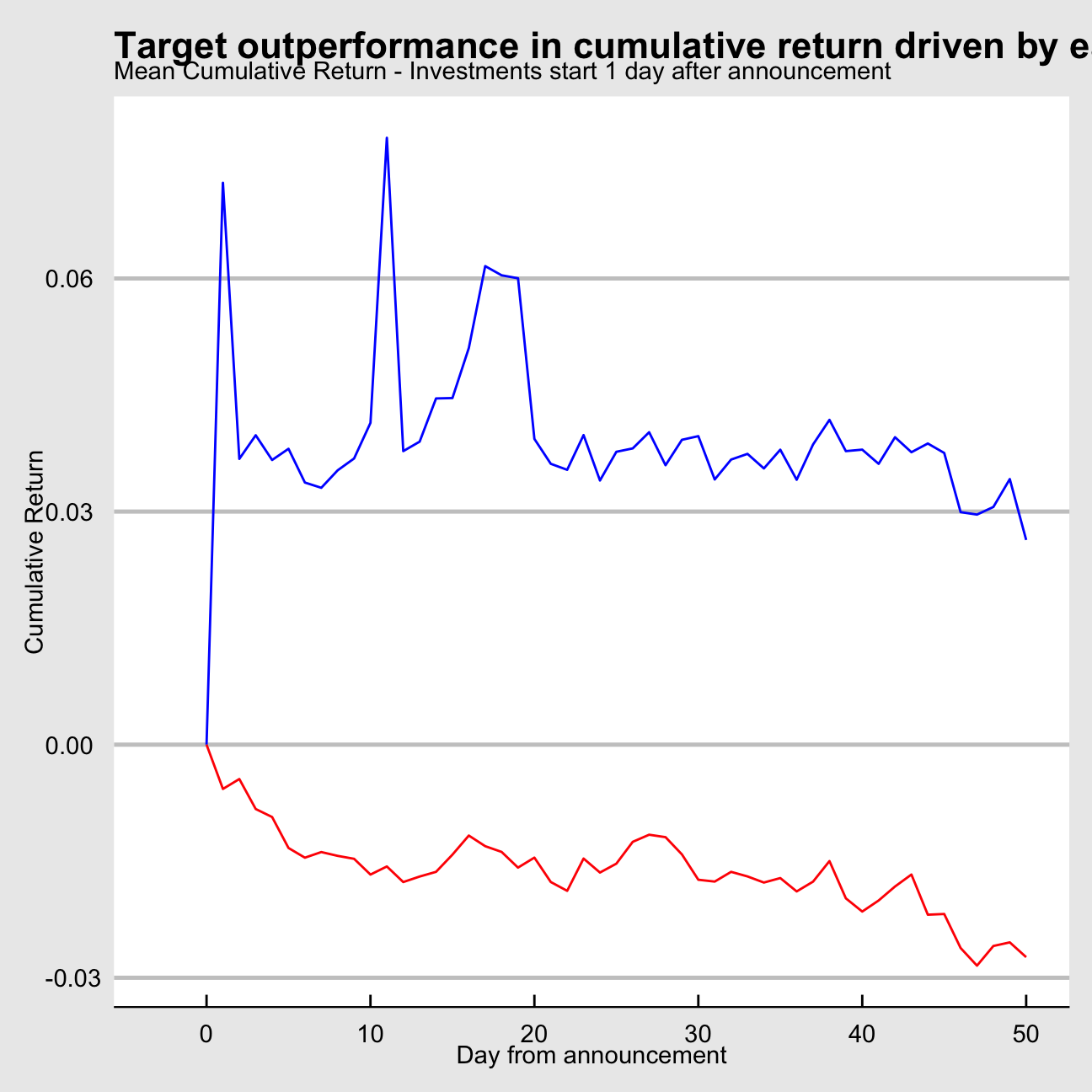
ggsave("Cumulative Returns Target and Acquirer.png",
       plot = last_plot(),
       scale = 1,
       width = 20,
       height = 15,
       units = "cm",
       dpi = 300,
       limitsize = TRUE)

knitr::include_graphics(here::here("Cumulative Returns Target and Acquirer.png"), error = FALSE)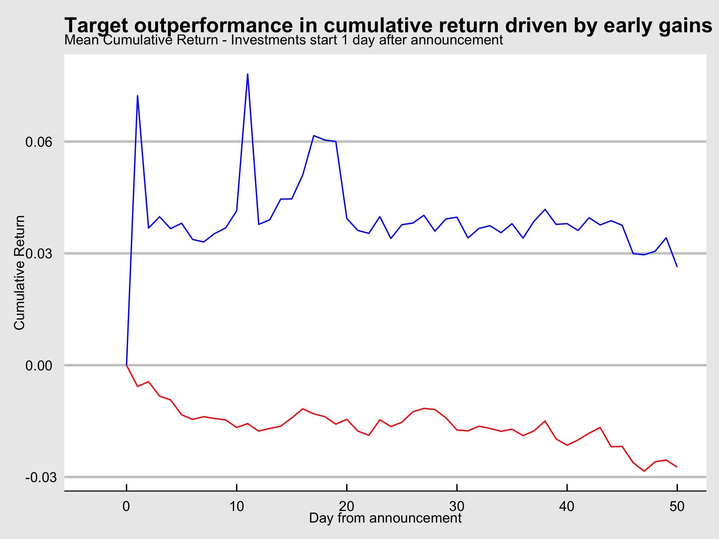
As we can see the majority of the spread is produced within the first five days from announcement, with the spread essentially staying flat from day 25 onwards.
Correlation between return and deal completion
Acquirer
end_acq <- acq_tar %>%
  mutate(diff = close_date - date) %>%
  filter(diff == 0) %>%
  rename(end_acq = close_acquirer) %>%
  select(acquirer, period, target, end_acq, DealStatus) %>%
  distinct()


deal_ret_acq <- left_join(end_acq, initial_acq, by = c("acquirer", "target")) %>%
  distinct() %>%
  mutate(annualised_ret = (end_acq/initial_acq)^(252/period) - 1) %>%
  group_by(DealStatus) %>%
  summarise(mean_annualised_acq_ret = median(annualised_ret, na.rm = TRUE))

deal_ret_acq| DealStatus | mean_annualised_acq_ret |
|---|---|
| Completed | -0.0129 |
| Failed | -0.46 |
end_tar <- acq_tar %>%
  mutate(diff = close_date - date) %>%
  filter(diff == 0) %>%
  rename(end_tar = close_target) %>%
  select(acquirer, period, target, end_tar, DealStatus) %>%
  distinct()


deal_ret_tar <- left_join(end_tar, initial_tar, by = c("acquirer", "target")) %>%
  filter(!is.na(end_tar)) %>%
  mutate(annualised_ret = (end_tar/initial_tar)^(252/period) - 1) %>%
  group_by(DealStatus) %>%
  summarise(mean_annualised_tar_ret = sprintf("%.2f",median(annualised_ret, na.rm = TRUE)))

deal_ret_tar| DealStatus | mean_annualised_tar_ret |
|---|---|
| Completed | 0.09 |
| Failed | -0.17 |
Huge failed deal target return driven by T - STRP deal, where STRP’s stock increased by 150% in 20 days.
Returns of strategy over timeline
From our analysis above we can find an arbitrage strategy that should yield risk-free returns by going long on target stocks and going short on acquirer stocks. Whereas we could protect ourselves from more risk by following a strategy closer to the one described in the economic rational chapter, longing and shorting the respective companies in a ratio as per the announced deal proposal, we follow a more simplified strategy for this project.
For every deal announced we will execute a long transaction for the target and a short transaction for the acquirer. In periods where deals overlap, we will assume an equal weighting in our investments, i.e. the strategy return will be the average of all targets’ and acquirers’ returns. For every time period without an active deal being in place, we will move our portfolio into the market, proxied by the S&P500 index.
Due to our difficulties of attaining target companies’ stock price data from Yahoo Finance for older deals we decided to use 01-01-2015 as our inception date for strategy. The majority of deals with good quality data are post this date which means we have less data-quality driven random fluctuations in our calculations.
As seen in the earlier section our performance spread between targets and acquirers narrows very quickly and hovers around 0% after 50 days. Due to our simplified nature of our strategy we want to avoid low spreads in later periods (post day 50) to neutralize high spreads of other deals in early periods if their dates happen to overlap. We therefore excluded all spready post day 50 from announcement.
S&P 500 if no deal
acq_tar2 <- acq_tar %>%
  filter(period <= 50) %>%
  group_by(date) %>%
  summarise(ret_strat = mean(ret_combined)) %>%
  filter(!is.na(ret_strat))


SP_initial <- benchmark %>%
  filter(description == "SP_500") %>%
  filter(date >= "2015-01-01") %>%
  arrange(date) %>%
  head(n = 1) %>%
  rename(initial_index = close) %>%
  select(- date, - index_return)

  ggplot(acq_tar2) +
geom_line(aes(x = date, y = ret_strat), colour = "red") 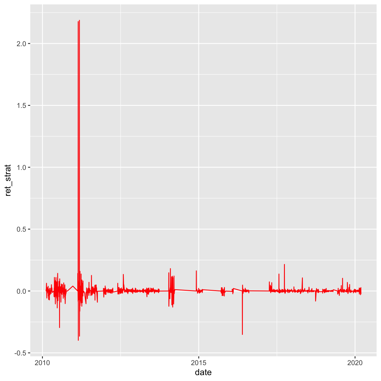
benchmark %>%
  filter(description == "SP_500") %>%
  arrange(date) %>%
  left_join(SP_initial, by = c("description", "index")) %>%
  left_join(acq_tar2, by = "date") %>%
  select(date, close, initial_index, ret_strat) %>%
  mutate(index_ret = close/lag(close) - 1,
         cum_index_ret = close/initial_index,
         ret_strat_adjusted = ifelse(is.na(ret_strat), index_ret, ret_strat)) %>%
  filter(date >= "2015-01-01") %>%
  mutate(retplus1 = ret_strat_adjusted + 1,
    cum_ret_strat = cumprod(retplus1)) %>%
  ggplot() +
  geom_line(aes(x = date, y = cum_index_ret), colour = "red") +
  geom_line(aes(x = date, y = cum_ret_strat), colour = "green") +
  labs(subtitle = "Cumulative Return Strategy vs Index",
       title = "Perfect Foresight Generates Above Market Returns",
       y = "Cumulative Return",
       x = "Day from initial investment") +
  theme_economist_white()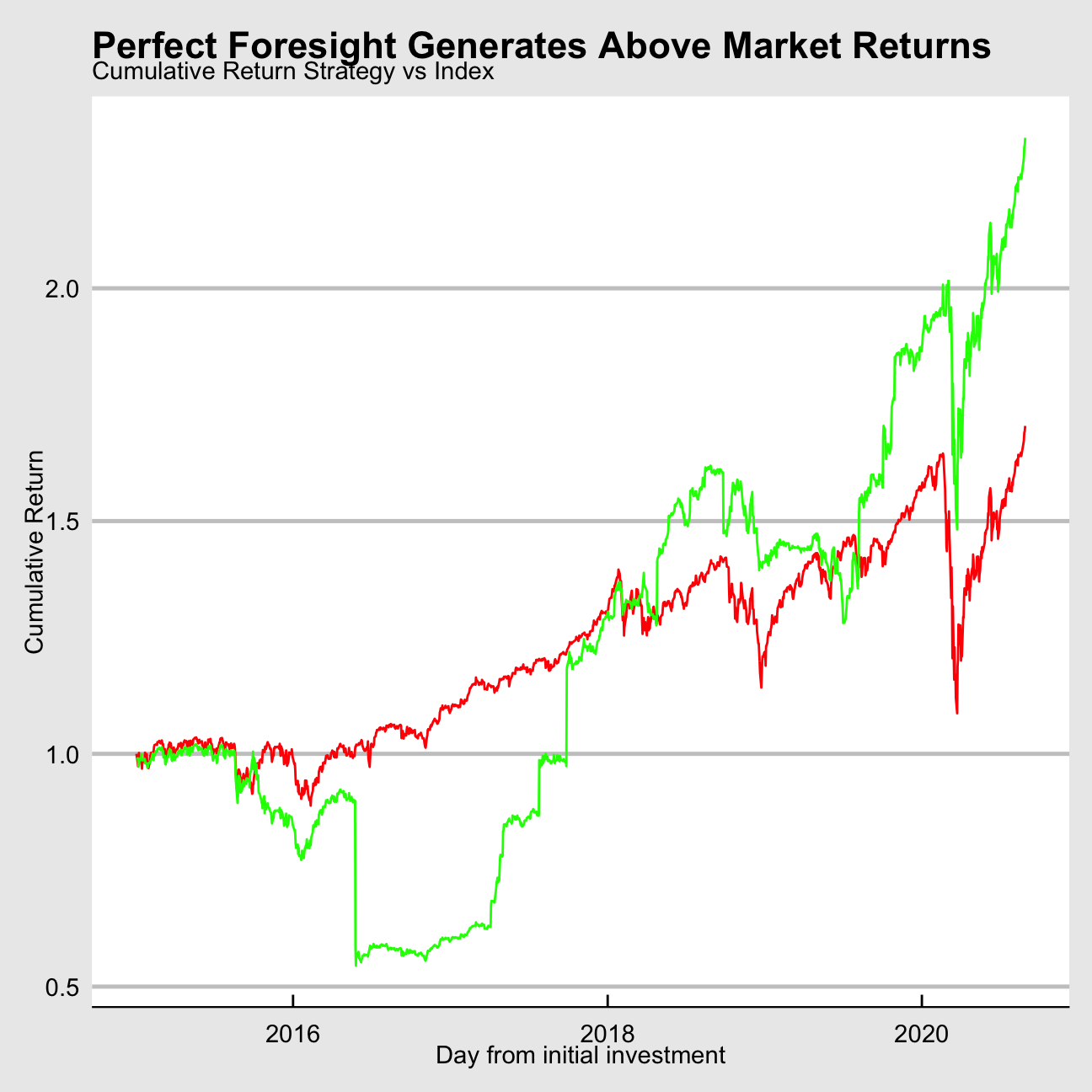
ggsave("Cumulative Return Strategy vs Index.png",
       plot = last_plot(),
       scale = 1,
       width = 20,
       height = 15,
       units = "cm",
       dpi = 300,
       limitsize = TRUE)

knitr::include_graphics(here::here("Cumulative Return Strategy vs Index.png"), error = FALSE)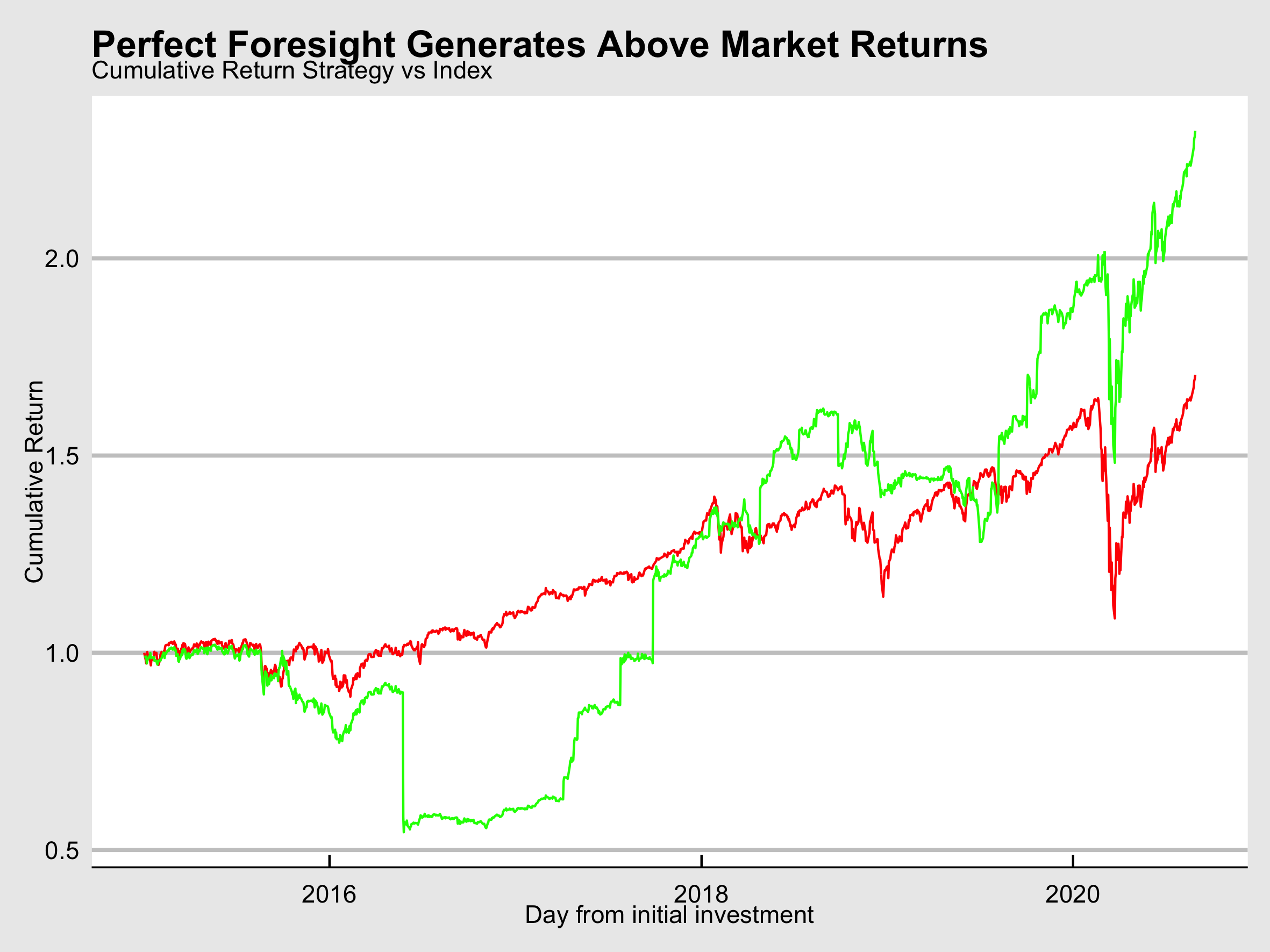
As can be seen in the chart above our strategy achieves extraordinary returns overall, with some steep price drops in between.
We can take away the following findings from this:
- On average the target-acquirer spread is positive and transacting on it before the market yields positive results.
- There are multiple occurrences of steep losses. Not all announcement will result in price increases for the target, nor the acquirer. An offer at a steep discount might result in the target’s stock price to crash. Our theoretical strategy as per the economic rational could hedge this risk, whilst also limiting the upside.
Risk free if no deal
benchmark %>%
  filter(description == "SP_500") %>%
  arrange(date) %>%
  left_join(SP_initial, by = c("description", "index")) %>%
  left_join(acq_tar2, by = "date") %>%
  left_join(tbill, by = "date") %>%
  select(date, close, initial_index, ret_strat, T_bill_d) %>%
  mutate(index_ret = close/lag(close) - 1,
         cum_index_ret = close/initial_index,
         ret_strat_adjusted = ifelse(is.na(ret_strat), T_bill_d, ret_strat)) %>%
  filter(date >= "2014-05-01") %>%
  mutate(retplus1 = ret_strat_adjusted + 1,
    cum_ret_strat = cumprod(retplus1)) %>%
  ggplot() +
  geom_line(aes(x = date, y = cum_index_ret), colour = "red") +
  geom_line(aes(x = date, y = cum_ret_strat), colour = "green") +
  labs(subtitle = "Cumulative Return Strategy vs Index",
       title = "Perfect Foresight Generates Above Market Returns",
       y = "Cumulative Return",
       x = "Day from initial investment") +
  theme_economist_white()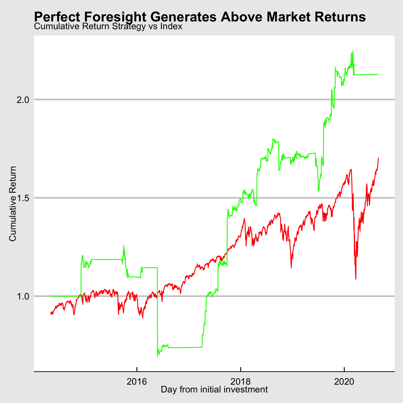
CAPM
To test the performance of our strategy in more detail we regressed our strategy’s excess returns to our benchmark’s (S&P500) excess return, where excess return means any return above the risk-free rate as per the respective 3-month US T-Bill
benchmarkSP <- benchmark %>%
  filter(description == "SP_500") %>%
  pivot_wider(values_from = index_return, names_from = description) %>%
  select(date, SP_500)


CAPM <- acq_tar %>%
  filter(period <= 20) %>%
  left_join(tbill, by = "date") %>%
  left_join(benchmarkSP, by = "date") %>%
  filter(!is.na(ret_combined)) %>%
  mutate(Rm_Rf = SP_500 - T_bill_d,
         Rs_Rf = ret_combined - T_bill_d) %>%  # CAN MUTATE RET_Strat = S&P/TBill if return = NA, then use that to replace ret_combined here
  drop_na(Rm_Rf, Rs_Rf) %>%
  filter(!is.infinite(Rs_Rf))

ggplot(CAPM, aes(x = Rm_Rf, y = Rs_Rf, na.rm = TRUE)) +
  geom_point() +
  geom_smooth(method = lm)  +
  ylim(-1,1) +
  labs(subtitle = "Excess Returns of Startegy vs Market Benchmark (scale ignoring 2 outliers)",
       title = "Regression shows minimal positive Alpha and Beta for daily returns",
       y = "Excess Return Strategy",
       x = "Excess Return Benchmark") +
  theme_economist_white()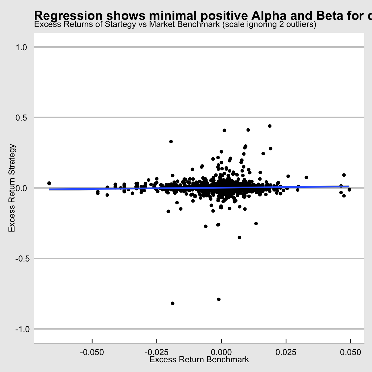
ggsave("Excess Returns of Startegy vs Market Benchmark.png",
       plot = last_plot(),
       scale = 1,
       width = 25,
       height = 15,
       units = "cm",
       dpi = 300,
       limitsize = TRUE)

knitr::include_graphics(here::here("Excess Returns of Startegy vs Market Benchmark.png"), error = FALSE)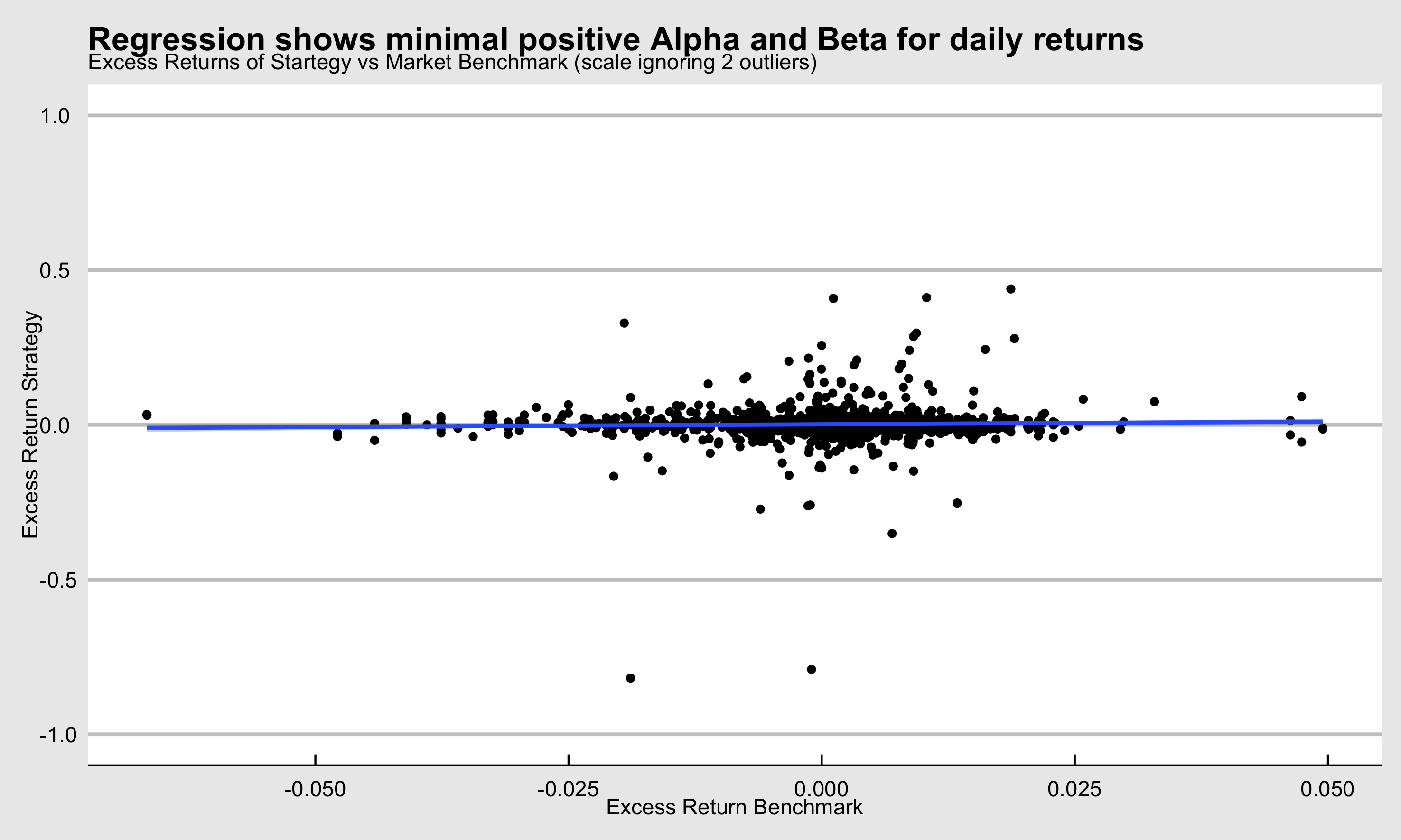
CAPM_regression <- lm(Rs_Rf ~ Rm_Rf, data = CAPM, na.rm =TRUE)

CAPM_regression
##
## Call:
## lm(formula = Rs_Rf ~ Rm_Rf, data = CAPM, na.rm = TRUE)
##
## Coefficients:
## (Intercept) Rm_Rf
## 0.005822 0.000526huxreg(CAPM_regression,
statistics = c('#observations' = 'nobs',
'R squared' = 'r.squared',
'Adj. R Squared' = 'adj.r.squared',
'Residual SE' = 'sigma'),
bold_signif = 0.05,
stars = NULL
)| (1) | |
|---|---|
| (Intercept) | 0.006 |
| (0.003) | |
| Rm_Rf | 0.001 |
| (0.311) | |
| #observations | 2213 |
| R squared | 0.000 |
| Adj. R Squared | -0.000 |
| Residual SE | 0.139 |
msummary(CAPM_regression)## Estimate Std. Error t value Pr(>|t|)
## (Intercept) 0.005822 0.002950 1.97 0.049 *
## Rm_Rf 0.000526 0.311403 0.00 0.999
##
## Residual standard error: 0.139 on 2211 degrees of freedom
## Multiple R-squared: 1.29e-09, Adjusted R-squared: -0.000452
## F-statistic: 2.85e-06 on 1 and 2211 DF, p-value: 0.999Our slope β not being statistically different from zero for our strategy is intuitive: for every deal we long and short one stock – every market related movement should be cancelled out. That being said, we still find a statistically significant alpha that is positive. On average our strategy, assuming perfect foresight, returns 0.87% daily unrelated to the market